Premier League Market Value Project

A project that uses Python to explore various factors of a dataset regarding Premier League soccer players.
The code below displays highlights from the project. For more details, please view the GitHub Repository.
Link to GitHub Repository:
Import data
#Step 1:  Load data into a dataframe
addr1 = "epldata_final.csv"
data = pd.read_csv(addr1)
# Step 2:  check the dimension of the table
print("The dimension of the table is: ", data.shape)

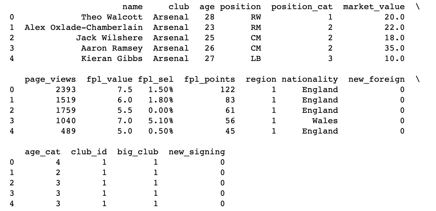
#Step 3:  Look at the data
print(data.head(5))
Explore Data
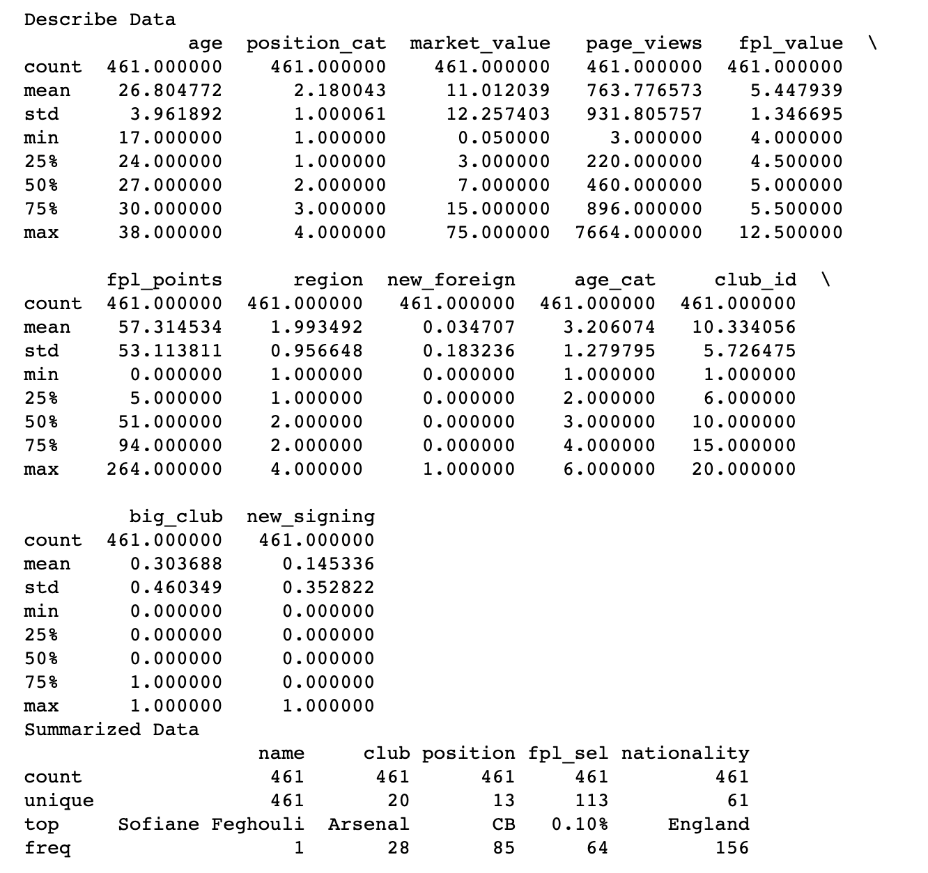
#Step 5:  what type of variables are in the table
print("Describe Data")
print(data.describe())
print("Summarized Data")
print(data.describe(include=['O']))
Data Visualization
#Step 6: import visulization packages
import matplotlib.pyplot as plt
# set up the figure size
plt.rcParams['figure.figsize'] = (20, 10)
# make subplots
fig, axes = plt.subplots(nrows = 2, ncols = 2)
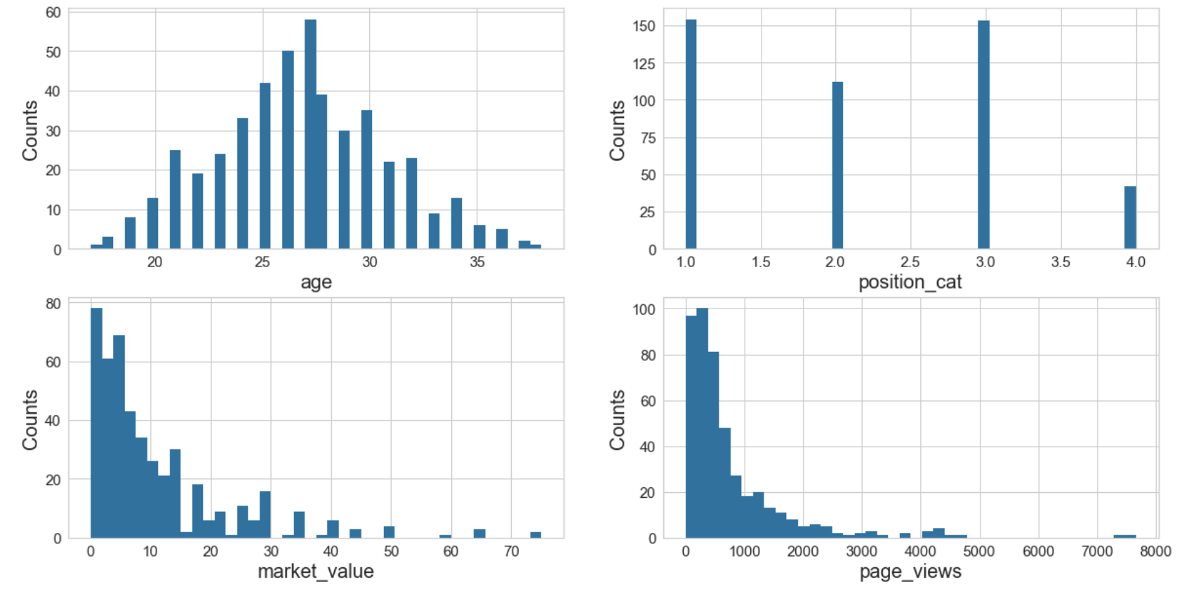
# Specify the features of interest
num_features = ['age', 'position_cat', 'market_value', 'page_views']
xaxes = num_features
yaxes = ['Counts', 'Counts', 'Counts', 'Counts']
# draw histograms
axes = axes.ravel()
for idx, ax in enumerate(axes):
ax.hist(data[num_features[idx]].dropna(), bins=40)
ax.set_xlabel(xaxes[idx], fontsize=20)
ax.set_ylabel(yaxes[idx], fontsize=20)
ax.tick_params(axis='both', labelsize=15)
plt.show()
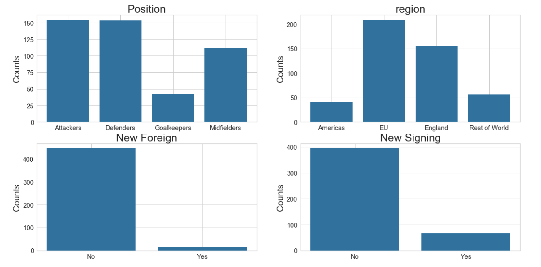
#7:  Barcharts: set up the figure size
#%matplotlib inline
plt.rcParams['figure.figsize'] = (20, 10)
# make subplots
fig, axes = plt.subplots(nrows = 2, ncols = 2)
# make the data read to feed into the visualizer
X_Position = data.replace({'position_cat': {1: 'Attackers', 2: 'Midfielders', 3: 'Defenders', 4: 'Goalkeepers'}}).groupby('position_cat').size().reset_index(name='Counts')['position_cat']
Y_Position = data.replace({'position_cat': {1: 'Attackers', 2: 'Midfielders', 3: 'Defenders', 4: 'Goalkeepers'}}).groupby('position_cat').size().reset_index(name='Counts')['Counts']
# make the bar plot
axes[0, 0].bar(X_Position, Y_Position)
axes[0, 0].set_title('Position', fontsize=25)
axes[0, 0].set_ylabel('Counts', fontsize=20)
axes[0, 0].tick_params(axis='both', labelsize=15)
# make the data read to feed into the visualizer
X_Region = data.replace({'region': {1: 'England', 2: 'EU', 3: 'Americas', 4: 'Rest of World'}}).groupby('region').size().reset_index(name='Counts')['region']
Y_Region = data.replace({'region': {1: 'England', 2: 'EU', 3: 'Americas', 4: 'Rest of World'}}).groupby('region').size().reset_index(name='Counts')['Counts']
# make the bar plot
axes[0, 1].bar(X_Region, Y_Region)
axes[0, 1].set_title('region', fontsize=25)
axes[0, 1].set_ylabel('Counts', fontsize=20)
axes[0, 1].tick_params(axis='both', labelsize=15)
# make the data read to feed into the visualizer
X_new_foreign = data.replace({'new_foreign':{0: 'No', 1: 'Yes'}}).groupby('new_foreign').size().reset_index(name='Counts')['new_foreign']
Y_new_foreign = data.replace({'new_foreign':{0: 'No', 1: 'Yes'}}).groupby('new_foreign').size().reset_index(name='Counts')['Counts']
# make the bar plot
axes[1, 0].bar(X_new_foreign, Y_new_foreign)
axes[1, 0].set_title('New Foreign', fontsize=25)
axes[1, 0].set_ylabel('Counts', fontsize=20)
axes[1, 0].tick_params(axis='both', labelsize=15)
# make the data read to feed into the visualizer
X_new_signing = data.replace({'new_signing':{0: 'No', 1: 'Yes'}}).groupby('new_signing').size().reset_index(name='Counts')['new_signing']
Y_new_signing = data.replace({'new_signing':{0: 'No', 1: 'Yes'}}).groupby('new_signing').size().reset_index(name='Counts')['Counts']
# make the bar plot
axes[1, 1].bar(X_new_signing, Y_new_signing)
axes[1, 1].set_title('New Signing', fontsize=25)
axes[1, 1].set_ylabel('Counts', fontsize=20)
axes[1, 1].tick_params(axis='both', labelsize=15)
plt.show()
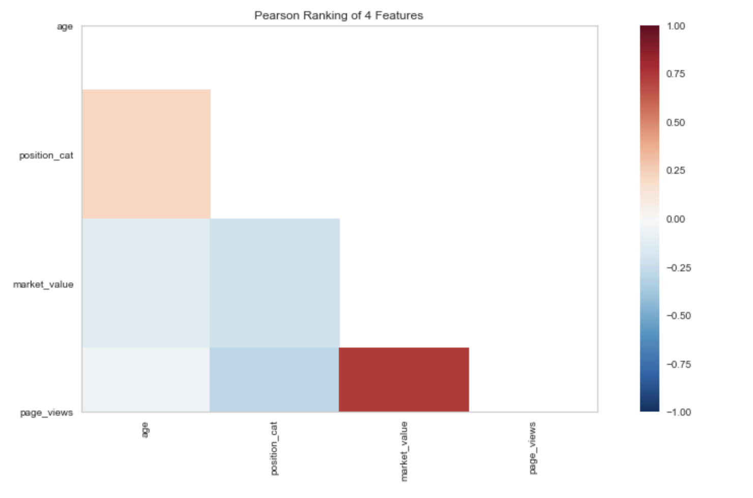
#Step 8: Pearson Ranking
#set up the figure size
#%matplotlib inline
plt.rcParams['figure.figsize'] = (15, 7)
# import the package for visulization of the correlation
from yellowbrick.features import Rank2D
# extract the numpy arrays from the data frame
X = data[num_features].values
# instantiate the visualizer with the Covariance ranking algorithm
visualizer = Rank2D(features=num_features, algorithm='pearson')
visualizer.fit(X)                # Fit the data to the visualizer
visualizer.transform(X)             # Transform the data
visualizer.poof(outpath="pcoords1.png") # Draw/show/poof the data
plt.show()
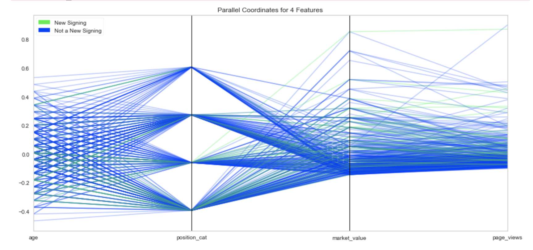
# Step 9:  Compare variables against New Signing and Not a New Signing
#set up the figure size
#%matplotlib inline
plt.rcParams['figure.figsize'] = (15, 7)
plt.rcParams['font.size'] = 50
# setup the color for yellowbrick visulizer
from yellowbrick.style import set_palette
set_palette('sns_bright')
# import packages
from yellowbrick.features import ParallelCoordinates
# Specify the features of interest and the classes of the target
classes = ['Not a New Signing', 'New Signing']
num_features = ['age', 'position_cat', 'market_value', 'page_views']
# copy data to a new dataframe
data_norm = data.copy()
# normalize data to 0-1 range
for feature in num_features:
    data_norm[feature] = (data[feature] - data[feature].mean(skipna=True)) / (data[feature].max(skipna=True) - data[feature].min(skipna=True))
# Extract the numpy arrays from the data frame
X = data_norm[num_features].as_matrix()
y = data.new_signing.as_matrix()
# Instantiate the visualizer
visualizer = ParallelCoordinates(classes=classes, features=num_features)
visualizer.fit(X, y)      # Fit the data to the visualizer
visualizer.transform(X)   # Transform the data
visualizer.poof(outpath="pcoords2.png") # Draw/show/poof the data
plt.show()
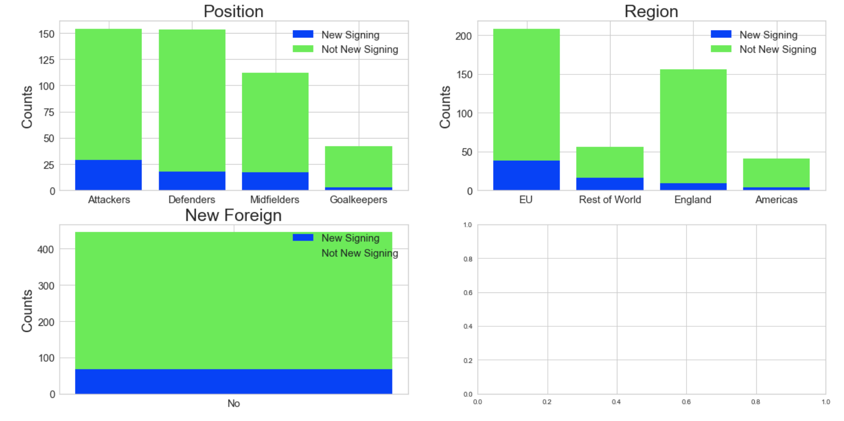
# Step 10 - stacked bar charts to compare new signing vs. not new signing
#set up the figure size
#%matplotlib inline
plt.rcParams['figure.figsize'] = (20, 10)
# make subplots
fig, axes = plt.subplots(nrows = 2, ncols = 2)
# make the data read to feed into the visualizer
Position_new_signing = data.replace({'new_signing': {1: 'New Signing', 0: 'Not New Signing'}}).replace({'position_cat': {1: 'Attackers', 2: 'Midfielders', 3: 'Defenders', 4: 'Goalkeepers'}})[data['new_signing']==1]['position_cat'].value_counts()
Position_not_new_signing = data.replace({'new_signing': {1: 'New Signing', 0: 'Not New Signing'}}).replace({'position_cat': {1: 'Attackers', 2: 'Midfielders', 3: 'Defenders', 4: 'Goalkeepers'}})[data['new_signing']==0]['position_cat'].value_counts()
Position_not_new_signing = Position_not_new_signing.reindex(index = Position_new_signing.index)
# make the bar plot
p1 = axes[0, 0].bar(Position_new_signing.index, Position_new_signing.values)
p2 = axes[0, 0].bar(Position_not_new_signing.index, Position_not_new_signing.values, bottom=Position_new_signing.values)
axes[0, 0].set_title('Position', fontsize=25)
axes[0, 0].set_ylabel('Counts', fontsize=20)
axes[0, 0].tick_params(axis='both', labelsize=15)
axes[0, 0].legend((p1[0], p2[0]), ('New Signing', 'Not New Signing'), fontsize = 15)


# make the data read to feed into the visualizer
region_new_signing = data.replace({'new_signing': {1: 'New Signing', 0: 'Not New Signing'}}).replace({'region': {1: 'England', 2: 'EU', 3: 'Americas', 4: 'Rest of World'}})[data['new_signing']==1]['region'].value_counts()
region_not_new_signing = data.replace({'new_signing': {1: 'New Signing', 0: 'Not New Signing'}}).replace({'region': {1: 'England', 2: 'EU', 3: 'Americas', 4: 'Rest of World'}})[data['new_signing']==0]['region'].value_counts()
region_not_new_signing = region_not_new_signing.reindex(index = region_new_signing.index)

# make the bar plot
p3 = axes[0, 1].bar(region_new_signing.index, region_new_signing.values)
p4 = axes[0, 1].bar(region_not_new_signing.index, region_not_new_signing.values, bottom=region_new_signing.values)
axes[0, 1].set_title('Region', fontsize=25)
axes[0, 1].set_ylabel('Counts', fontsize=20)
axes[0, 1].tick_params(axis='both', labelsize=15)
axes[0, 1].legend((p3[0], p4[0]), ('New Signing', 'Not New Signing'), fontsize = 15)

# make the data read to feed into the visualizer
new_foreign_new_signing = data.replace({'new_signing': {1: 'New Signing', 0: 'Not New Signing'}}).replace({'new_foreign': {0: 'No', 1: 'Yes'}})[data['new_signing']==1]['new_foreign'].value_counts()
new_foreign__not_new_signing = data.replace({'new_signing': {1: 'New Signing', 0: 'Not New Signing'}}).replace({'new_foreign': {0: 'No', 1: 'Yes'}})[data['new_signing']==0]['new_foreign'].value_counts()
new_foreign__not_new_signing = new_foreign__not_new_signing.reindex(index = new_foreign_new_signing.index)
# make the bar plot
p5 = axes[1, 0].bar(new_foreign_new_signing.index, new_foreign_new_signing.values)
p6 = axes[1, 0].bar(new_foreign__not_new_signing.index, new_foreign__not_new_signing.values, bottom=new_foreign_new_signing.values)
axes[1, 0].set_title('New Foreign', fontsize=25)
axes[1, 0].set_ylabel('Counts', fontsize=20)
axes[1, 0].tick_params(axis='both', labelsize=15)
axes[1, 0].legend((p5[0], p6[0]), ('New Signing', 'Not New Signing'), fontsize = 15)

plt.show()
Prepare data for machine learning algorithms
# Step 11 - fill in missing values and eliminate features
#fill the missing age data with median value
def fill_na_median(data, inplace=True):
return data.fillna(data.median(), inplace=inplace)
fill_na_median(data['age'])
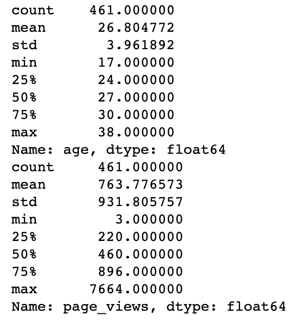
# check the result
print(data['age'].describe())
# fill with the most represented value
def fill_na_most(data, inplace=True):
return data.fillna('S', inplace=inplace)
fill_na_most(data['page_views'])
# check the result
print(data['page_views'].describe())
# import package
import numpy as np
# log-transformation
def log_transformation(data):
return data.apply(np.log1p)
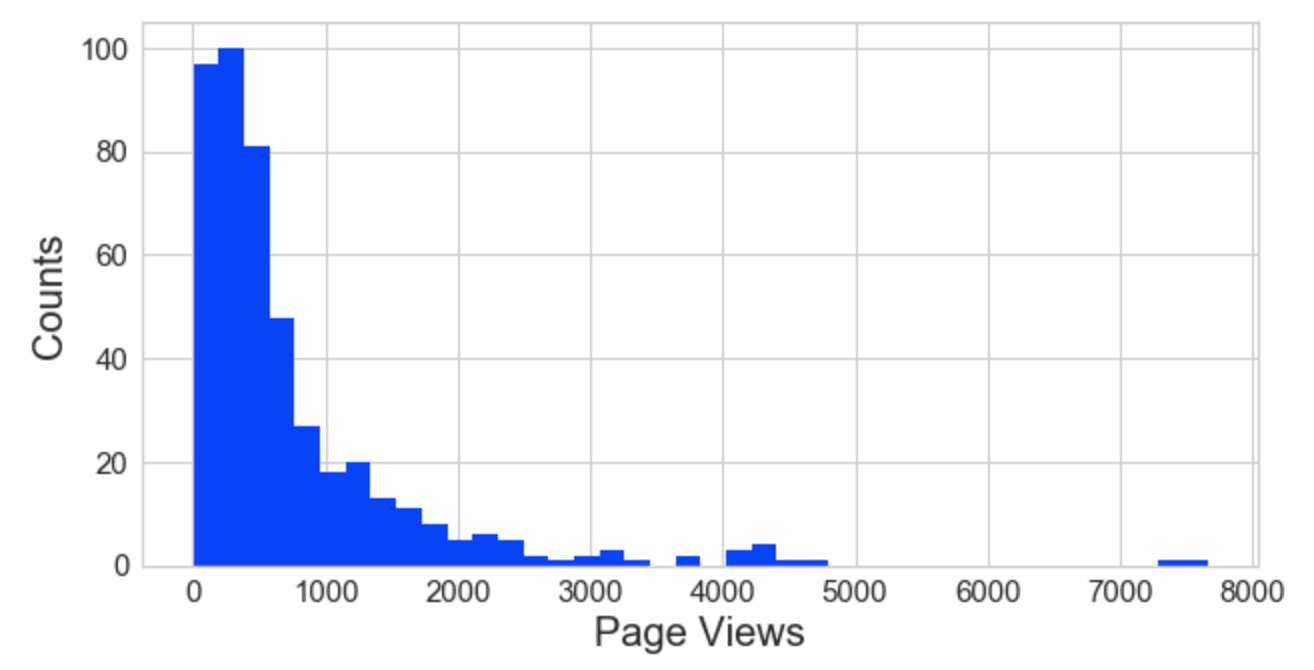
#Step 12 - adjust skewed data (fare)
#check the distribution using histogram
# set up the figure size
%matplotlib inline
plt.rcParams['figure.figsize'] = (10, 5)

plt.hist(data['page_views'], bins=40)
plt.xlabel('Page Views', fontsize=20)
plt.ylabel('Counts', fontsize=20)
plt.tick_params(axis='both', labelsize=15)
plt.show()
#Step 13 - convert categorical data to numbers
#get the categorical data
cat_features = ['position_cat', 'age', "market_value", 'page_views', 'fpl_value', 'fpl_points', 'region', 'new_foreign', 'new_signing']
data_cat = data[cat_features]
data_cat = data_cat.replace({'position_cat': {1: 'Attackers', 2: 'Midfielders', 3: 'Defenders', 4: 'Goalkeepers'}})
data_cat_2 = data_cat.replace({'region': {1: 'England', 2: 'EU', 3: 'Americas', 4: 'Rest of World'}})
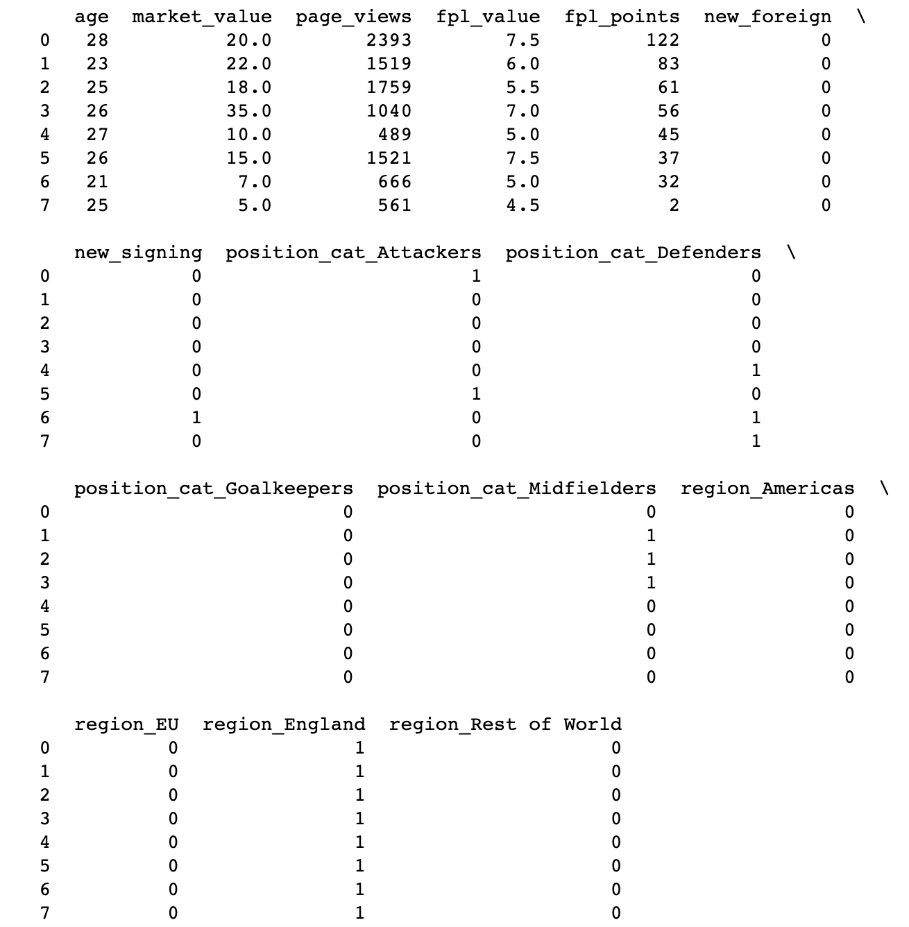
# One Hot Encoding
data_cat_dummies = pd.get_dummies(data_cat_2)
# check the data
# print(data_cat_dummies.head(8))
print(data_cat_dummies[:8])
import numpy as np
from sklearn.linear_model import LogisticRegression
from sklearn import datasets
from sklearn.model_selection import train_test_split
from sklearn.preprocessing import StandardScaler
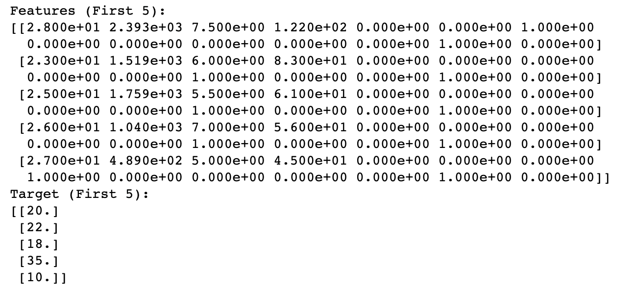
features = data_cat_dummies[['age', 'page_views', 'fpl_value', 'fpl_points', 'new_foreign', 'new_signing', 'position_cat_Attackers',
'position_cat_Defenders', 'position_cat_Goalkeepers', 'position_cat_Midfielders', 'region_Americas',
'region_EU', 'region_England', 'region_Rest of World']].values
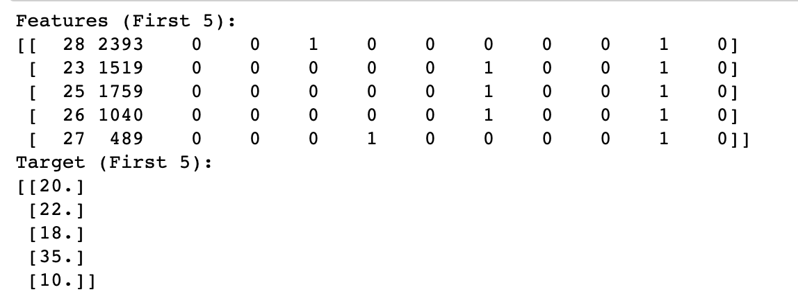
print ('Features (First 5):')
print(features[:5])
target = data_cat_dummies[['market_value']].values
print('Target (First 5):')
print(target[:5])
features_train, features_test, target_train, target_test = train_test_split(features, target, test_size=0.3, random_state=0)
#standardize features
# Create a scaler object
sc = StandardScaler()
# Fit the scaler to the training data and transform
features_train_std = sc.fit_transform(features_train)

# Apply the scaler to the test data
features_test_std = sc.transform(features_test)

from sklearn import preprocessing
lab_enc = preprocessing.LabelEncoder()
target_train_encoded = lab_enc.fit_transform(target_train)
target_test_encoded = lab_enc.fit_transform(target_test)

#Run LR with L1 at various strengths ******NOTE - change to L2 for second run!
C = [10, 1, .1, .001]

for c in C:
    clf = LogisticRegression(penalty='l1', C=c)
    clf.fit(features_train, target_train_encoded)
    print('C:', c)
    print('Coefficient of each feature:', clf.coef_)
    print('Training accuracy:', clf.score(features_train, target_train_encoded))
    print('Test accuracy:', clf.score(features_test, target_test_encoded))
    print('')

    # Based on previous results, removing the Fantasy features and increasing the Training set to 85% to see if this improves results

features_2 = data_cat_dummies[['age', 'page_views', 'new_foreign', 'new_signing', 'position_cat_Attackers',
                'position_cat_Defenders', 'position_cat_Goalkeepers', 'position_cat_Midfielders', 'region_Americas',
                'region_EU', 'region_England', 'region_Rest of World']].values
print ('Features (First 5):')
print(features_2[:5])
target_2 = data_cat_dummies[['market_value']].values
print('Target (First 5):')
print(target_2[:5])