Salary Forecasting with Predictive Analytics

A project that explores the trends of salaries for a variety of positions and uses machine learning algorithms to see if salary trends can be predicted for these roles and by region.

The code below displays highlights from the project. For more details, please view the GitHub Repository.

Link to GitHub Repository:

Click Here

Data Exploration in Python

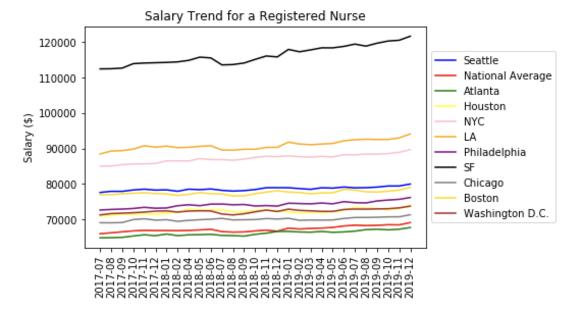
# Compare Registered Nurse salary trends across regions
x = df_SEA_RN.Month
y = df_SEA_RN.Value
z = df_US_RN.Value
a = df_ATL_RN.Value
b = df_HOU_RN.Value
c = df_NYC_RN.Value
d = df_LA_RN.Value
e = df_PHIL_RN.Value
f = df_SF_RN.Value
g = df_CHI_RN.Value
h = df_BOS_RN.Value
i = df_DC_RN.Value

plt.plot(x,y, color='blue')
plt.plot(x,z, color='red')
plt.plot(x,a, color='green')
plt.plot(x,b, color='yellow')
plt.plot(x,c, color='pink')
plt.plot(x,d, color='orange')
plt.plot(x,e, color='purple')
plt.plot(x,f, color='black')
plt.plot(x,g, color='gray')
plt.plot(x,h, color='gold')
plt.plot(x,i, color='brown')

plt.xticks(rotation=90)
plt.ylabel('Salary ($)')
plt.title('Salary Trend for a Registered Nurse')
plt.legend(['Seattle', 'National Average', 'Atlanta', 'Houston', 'NYC', 'LA', 'Philadelphia', 'SF', 'Chicago', 'Boston', 'Washington D.C.'],loc='center left', bbox_to_anchor=(1, 0.5))
plt.show

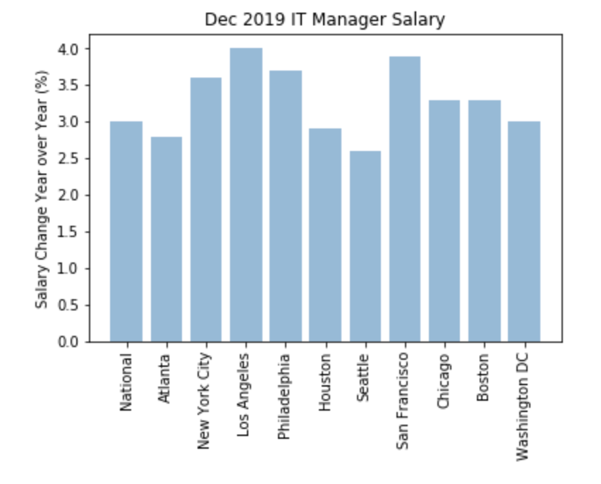
# Compare YoY values for Dec 2019 IT Manager across regions
objects = df_IT_Manager_1219.Metro
y_pos = np.arange(len(objects))
performance = df_IT_Manager_1219.YoY

plt.bar(y_pos, performance, align='center', alpha=0.5)
plt.xticks(y_pos, objects, rotation=90)
plt.ylabel('Salary Change Year over Year (%)')
plt.title('Dec 2019 IT Manager Salary')

plt.show()

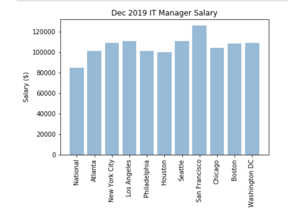
# Plot the salaries for IT Manager for Dec 2019 across regions
import numpy as np

objects = df_IT_Manager_1219.Metro
y_pos = np.arange(len(objects))
performance = df_IT_Manager_1219.Value

plt.bar(y_pos, performance, align='center', alpha=0.5)
plt.xticks(y_pos, objects, rotation=90)
plt.ylabel('Salary ($)')
plt.title('Dec 2019 IT Manager Salary')

plt.show()

Neural Network in Python

# Import data
train = pd.read_csv('df_all_final.csv')
# In the original export, an additional column for index values was added so that needs to be removed.
# Removing other columns not needed for analysis
train = train.drop(["Unnamed: 0","Metro","Dimension Type","Dimension","Measure","Value"], axis = 1)
# Review data
train.shape

# Create X variable for features and Y variable for target
X = train.drop('Value_bins', axis=1) #features
y = train['Value_bins'] #target
# Train and Test Split
X_train, X_test, y_train, y_test = train_test_split(X, y, test_size = 0.2, random_state = 42)
# Applying standard scaling
sc = StandardScaler()
X_train = sc.fit_transform(X_train)
X_test = sc.transform(X_test)
# Create multilayer perceptron neural network
mlpc = MLPClassifier(hidden_layer_sizes=(25,25,25,25,25), max_iter=1000)
mlpc.fit(X_train, y_train)
pred_mlpc = mlpc.predict(X_test)
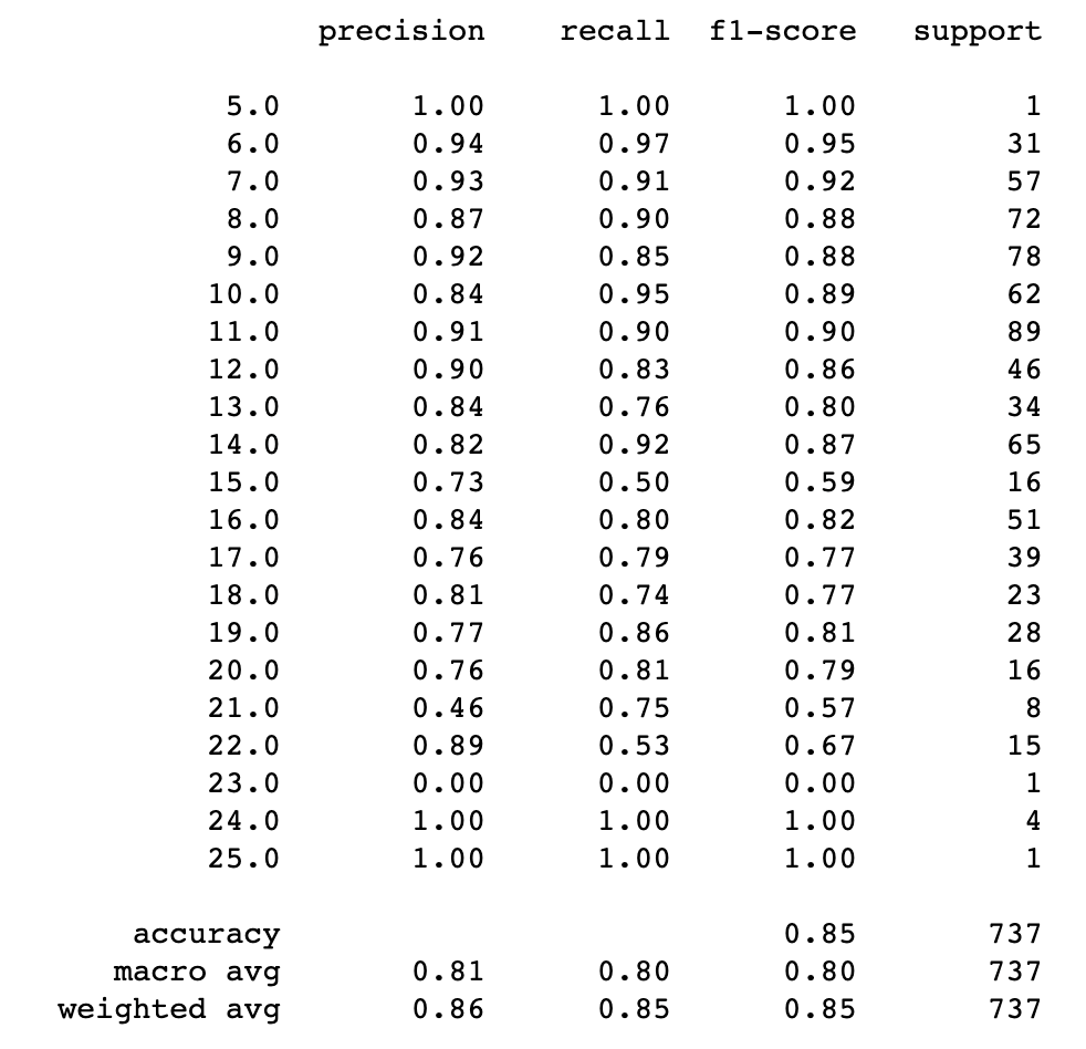
# Display classification report
print(classification_report(y_test, pred_mlpc))
# Calculate accuracy of model
cm = accuracy_score(y_test, pred_mlpc)
print("Model Accuracy: "+"{:.2%}".format(cm))

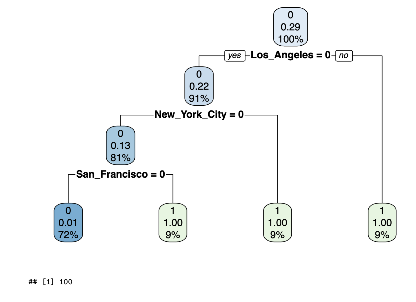
Decision Tree in R

Import data and libraries

library(rpart)
library(rpart.plot)
data_RN = read.csv("df_RN.csv", header = TRUE)

Build function for Decision Tree Model

decision_tree_job_title <- function(data){
  data_updated <- data.frame(data$Month,data$YoY,data$Atlanta,data$Boston,data$Chicago,data$Houston,data$Los.Angeles,data$National,data$New.York.City,data$Philadelphia,data$San.Francisco,data$Seattle,data$Washington.DC,data$Value_split)
  names(data_updated) <- c("Month","YoY","Atlanta","Boston","Chicago","Houston","Los_Angeles","National","New_York_City","Philadelphia","San_Francisco","Seattle","Washington_DC","Value_split")
  ran <- sample(1:nrow(data_updated), 0.9 * nrow(data_updated))
  nor <-function(x) { (x -min(x))/(max(x)-min(x)) }
  train_norm <- as.data.frame(lapply(data_updated, nor))
  data_train <- train_norm[ran,]
  data_test <- train_norm[-ran,]
  dtm <- rpart(Value_split~., data_train, method="class")
  rpart.plot(dtm, compress=TRUE, uniform=TRUE)
  p <- predict(dtm, data_test, type="class")
  confMat <- table(data_test$Value_split,p)
  accuracy <- sum(diag(confMat))/sum(confMat)
  return (accuracy*100)
}

Run Decision Tree

decision_tree_job_title(data_RN)